Tag Archives: FFT

Resolution of Discrete Fourier Transform

In the previous post we had introduced the Discrete Fourier Transform (DFT) as a method to perform the spectral analysis of a time domain signal. We now discuss an important property of the DFT, its spectral resolution i.e. its ability to resolve two signals with similar spectral content.

Initially one might think that increasing the sampling frequency would increase the spectral resolution but this totally incorrect. In fact if the sampling frequency is increased, keeping the number of time domain samples to be the same, the resolution actually decreases. So how do we calculate the spectral resolution. One simple way is to calculate the difference between two frequency bins as fs/(N-1) or 1/(N-1)Ts. Simply put the resolution in the frequency domain is the inverse of the sample length in the time domain.

So let us now calculate the DFT of two closely spaced sine waves keeping the sampling frequency to be the same and changing the number of time domain samples (only the result for N=64 shown here). We again list down the code used to calculate the DFT.

clear all
close all

fm1=100;
fm2=120;
fs=1000;
Ts=1/fs;
N=64;
t=0:Ts:(N-1)*Ts;

x1=cos(2*pi*fm1*t);
x2=cos(2*pi*fm2*t);
x=x1+x2;
W=exp(-j*2*pi/N);

n=0:N-1;
k=0:N-1;

X=x*(W.^(n'*k));

plot(k/N,abs(X))
xlabel ('Normalized Frequency')
ylabel ('X')

We first do some quick math to find the spectral resolution.

 fs/(N-1)=1000/(64-1)=15.87 Hz

Now the two tones are space 20 Hz apart (100 Hz and 120 Hz), so we can predict that the two tones would be detected successfully. The result of the DFT operation on the composite signal is shown below.
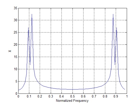
DFT of Two Tones
DFT of Two Tones

It is observed that although the two tones are detected, they are not exactly at the desired frequencies (0.10 and 0.12). Secondly the amplitude of the two tones is different although the time domain signals had equal amplitude. Both these phenomenon are due to the fact that we only have a limited number of frequency bins (N=64) due to which the resulting spectrum is only an estimate of the true spectrum.

There are better techniques than DFT to separate two closely spaced sinusoids and these are known as super resolution spectral techniques and would be discussed some other time.
Discrete Fourier Transform

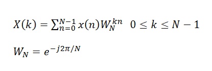
Discrete Fourier Transform or DFT is a mathematical operation that transforms a time domain signal to frequency domain. It is usually implemented using the Fast Fourier Transform (FFT). The computational complexity of the DFT is N2 whereas its (N)log2N for the FFT, where N is the number of samples of the the time domain signal. Mathematically, the DFT is written as

and this operation can be easily implemented in MATLAB as shown below.

clear all
close all

fm=100;
fs=1000;
Ts=1/fs;
N=1024;
t=0:Ts:(N-1)*Ts;

x=cos(2*pi*fm*t);
W=exp(-j*2*pi/N);

n=0:N-1;
for k=0:N-1
        X(k+1)=sum(x.*(W.^(k*n)));
end

plot((0:k)/N,abs(X))
xlabel ('Normalized Frequency')
ylabel ('X')

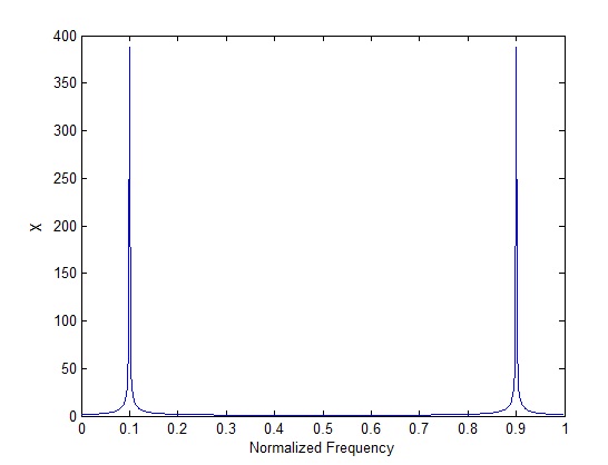
The DFT of the cosine function with frequency of 100Hz is shown below. It must be noted that the frequency in the figure below is normalized by the sampling frequency. So the peaks in the graph occur at 0.1*1000=100Hz and 0.9*1000=900Hz (image frequency). Actually if you zoom in you will see that the peaks are not exactly at 0.1 and 0.9 but  are slightly offset as the frequency bins are not located at exactly those frequencies.

DFT of a cosine wave

In case of multiple sinusoids the resolution of the DFT becomes important. Higher the sample size (duration of the time domain signal) higher is the resolution of the DFT. As stated earlier the DFT is a computationally complex operation and usually the Fast Fourier Transform (FFT) is used to compute the frequency domain behavior. We will discuss this in the following posts.

A simple way to expedite the process of DFT calculation is to use matrix manipulation instead of a “for loop”.This is shown below.

clear all
close all

fm=100;
fs=1000;
Ts=1/fs;
N=128;
t=0:Ts:(N-1)*Ts;

x=cos(2*pi*fm*t);
W=exp(-j*2*pi/N);

n=0:N-1;
k=0:N-1;

X=x*(W.^(n'*k));

plot(k/N,abs(X))
xlabel ('Normalized Frequency')
ylabel ('X')

Although matrix manipulation makes for a nice and clean code, it was found that there was no improvement in the computation time. Both the “for loop” code and the “matrix multiplication” code took about 0.35 seconds to execute. However, increasing the sample size from 128 to 1024 results in significant better computation time for the latter scheme.