Just to recap, building an LTE fading simulator with the desired temporal and spatial correlation is a three step procedure.
1. Generate Rayleigh fading sequences using Smith’s method which is based on Clarke and Gan’s fading model.
2. Introduce spatial correlation based upon the spatial correlation matrices defined in 3GPP 36.101.
3. Use these spatially and temporally correlated sequences as the filter taps for the LTE channel models.
We have already discussed step 1 and 3 in our previous posts. We now focus on step 2, generating spatially correlated channels coefficients.
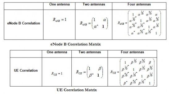
3GPP has defined spatial correlation matrices for the Node-B and the UE. These are defined for 1,2 and 4 transmit and receive antennas. These are reproduced below.
The parameters ‘alpha’ and ‘beta’ are defined as:
Low Correlation
alpha=0, beta=0
Medium Correlation
alpha=0.3, beta=0.9
High Correlation
alpha=0.9, beta=0.9
The combined effect of antenna correlation at the transmitter and receiver is obtained by taking the Kronecker product of individual correlation matrices e.g. for a 2×2 case the correlation matrix is given as:
Multiplying the square root of the correlation matrix with the vector of channel coefficients is equivalent to taking a weighted average e.g. for the channel between transmit antenna 1 and receive antenna 1 the correlated channel coefficient h11corr is given as:
h11corr=w1*h11+w2*h12+w3*h21+w4*h22
where w1=1 and w2, w3 and w4 are less than one and greater than zero. For the high correlation case described above the channel coefficient is calculated as:
h11corr=0.7179*h11+0.4500*h12+0.4500*h21+0.2821*h22
From a practical point of antenna correlation is dependent on the antenna separation. Greater the antenna spacing lower is the antenna correlation and better the system performance. However, a base station requires much higher antenna spacing than a UE to achieve the same level of antenna correlation. This is due to the fact the base station antennas are placed much higher than a UE. Therefore the signals arriving at the base station are usually confined to smaller angles and experience similar fading. A UE on the other hand has a lot of obstacles in the surrounding areas which results in higher angle spread and uncorrelated fading between the different paths.
Author: Yasir
More than 20 years of experience in various organizations in Pakistan, the USA, and Europe. Worked with the Mobile and Portable Radio Group (MPRG) of Virginia Tech and Qualcomm USA and was one of the first researchers to propose Space Time Block Codes for eight transmit antennas. Have publsihed a book “Recipes for Communication and Signal Processing” through Springer Nature.


9 thoughts on “A Rayleigh Fading Simulator with Temporal and Spatial Correlation”
give me the best open source free software for lte downlink scheduling performance measurement.
Hello,
First of all, many thanks for your blog and your efforts to explain all those topics with huge details and examples, it is really a very useful site.
I have one question regarding the 4 antennas case correlation matrix.
To simplify , let’s take the 1*4 case. We have to compute the sqrtm of this matrix.
But then, if we compare the sum of the applied weigths for the different correlated channels, they are not identical. As a result, we will have a difference in terms of received power at the 4 distinct receive antennas. I assume one additional normalization is needed, right ?
Thank you in advance for your advice and feeback.
Best regards,
Lo
Hi!
I am trying to build a LTE simulator with 2×2 MIMO. My problem is that I do not know where to use high,where to use medium and where to use low correlation matrices.
Normaly for LOS the correlation should be high (usualy you cannot do spatial multiplexing for LOS) and for NLOS lower.
Can I find this information in some standards?Any suggestions?
Regards,
I have looked at 3GPP TS36.101 v11.3.0 but it does not discuss the details of the scenarios.
John
hello John ,
I guess you took the case where the matrix is given by:
1.0000 0.9000 0.9000 0.8100
0.9000 1.0000 0.8100 0.9000
0.9000 0.8100 1.0000 0.9000
0.8100 0.9000 0.9000 1.0000
I used the sqrtm() function in matlab to get the square root of this matrix and it is given by :
0.7179 0.4500 0.4500 0.2821
0.4500 0.7179 0.2821 0.4500
0.4500 0.2821 0.7179 0.4500
0.2821 0.4500 0.4500 0.7179
in this case
h11corr= 0.7179*h11+0.4500*h12+0.4500 *h21+0.2821*h22
and effectively E[h11corr*h11corr]= 1
I think you used sqrt(Matrix) instead of sqrtm(Matrix) 🙂
Thanks for your fast reply, and thanks again, your site it is wonderfull.
Correction made. Thanks!
Ali: I am really happy to see that somebody has looked into this post in so much detail. I totally agree with what you have said and have made the correction. Please let me know if this makes sense now.
Hello,
First I would like to thank you for your blog and for your effort, it is really great website.
Second I would like to make some commentary about the proposed method, well the method is not so clear, but I guess you propose to generate a vector of 4 channels seperately using the Jakes method that represents the 2X2 MIMO and then to multiply it by the matrix Rspat.
Well this wouldn’t generate the right spatial correlation, this can be simply verified by computing: E[Chan1*Chan1] with Chan1 =h11+0.9*h12+0.9*h21+0.81*h22, the result would not be one.
I think that the right method is to generate a vector of 4 channels seperately using the Jakes method then to multiply it by the root square of matrix Rspat.
I am waiting your feedback.
Best Regards,
Ali
Impressive stuff.