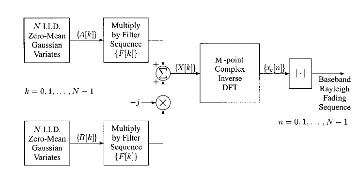
We had previously presented a method of generating a temporally correlated Rayleigh fading sequence. This was based on Smith’s fading simulator which was based on Clark and Gan’s fading model. We now present a highly efficient method of generating a correlated Rayleigh fading sequence, which has been adapted from Young and Beaulieu’s technique [1]. The architecture of this fading simulator is shown below.

This method essentially involves five steps.

1. Generate two Gaussian random sequences of length N each.
2. Multiply these sequences by the square root of Doppler Spectrum S=1.5./(pi*fm*sqrt(1-(f/fm).^2).
3. Add the two sequences in quadrature with each other to generate a length N complex sequence (we have added the two sequences before multiplying with the square root of Doppler Spectrum in our simulation).
4. Take the M point complex inverse DFT where M=(fs/Δf)+1.
5. The absolute value of the resulting sequence defines the envelope of the Rayleigh faded signal with the desired temporal correlation (based upon the Doppler frequency fm).

A point to be noted here is that although the Doppler spectrum is defined from -fm to +fm the IDFT has to be taken from -fs/2 to +fs/2. This is achieved by stuffing zeros in the vacant frequency bins from -fs/2 to +fs/2. The MATLAB code for this simulator is given below.

%%%%%%%%%%%%%%%%%%%%%%%%%%%%%%%%%%%%%%%%%%%%%%%%%%%%%%%%%%%%%%%%%%%%%%%%%%
% RAYLEIGH FADING SIMULATOR BASED UPON YOUNG'S METHOD
% N is the number of paths
% M is the total number of points in the frequency domain
% fm is the Doppler frequency in Hz
% fs is the sampling frequency in Hz
% df is the step size in the frequency domain
% Copyright RAYmaps (www.raymaps.com)
%%%%%%%%%%%%%%%%%%%%%%%%%%%%%%%%%%%%%%%%%%%%%%%%%%%%%%%%%%%%%%%%%%%%%%%%%%
clear all;
close all;                          
 
N=64;
fm=70;
df=(2*fm)/(N-1);
fs=7.68e6;
M=round(fs/df);
T=1/df;
Ts=1/fs;                                
 
% Generate 2xN IID zero mean Gaussian variates
g1=randn(1,N);  
g2=randn(1,N);
g=g1-j*g2;                              
 
% Generate Doppler Spectrum
f=-fm:df:fm;
S=1.5./(pi*fm*sqrt(1-(f/fm).^2));
S(1)=2*S(2)-S(3);
S(end)=2*S(end-1)-S(end-2);        
 
% Multiply square root of Doppler Spectrum with Gaussian random sequence
X=g.*sqrt(S);

% Take IFFT
F_zero=zeros(1, round((M-N)/2));
X=[F_zero, X, F_zero];
x=ifft(X,M);
r=abs(x);
r=r/mean(r);                        
 
% Plot the Rayleigh envelope
t=0:Ts:T-Ts;
plot(t,10*log10(r))
xlabel('Time(sec)')
ylabel('Signal Amplitude (dB)')
%%%%%%%%%%%%%%%%%%%%%%%%%%%%%%%%%%%%%%%%%%%%%%%%%%%%%%%%%%%%%%%%%%%%%%%%%%

The question now is that how do we verify that the generated Rayleigh fading sequence has the desired statistical properties. This can be verified by looking at the level crossing rate (LCR) and average fade duration (AFD) of the generated sequence as well as the PDF and Autocorrelation function. The LCR and AFD calculated for N=64 and fm=70 Hz and threshold of -10 dB (relative to the average signal power) is given below.

LCR
Simulation: 15.55
Theoretical: 15.46

AFD
Simulation: 453 usec
Theoretical:  508 usec

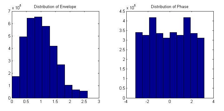
It is observed that the theoretical and simulation results for the LCR and AFD match reasonably well. We next examine the distribution of the envelope and phase of the resulting sequence x. It is found that the envelope of x is Rayleigh distributed while the phase is uniformly distributed from -pi to pi. This is shown in the figure below. So we are reasonably satisfied that our generated sequence has the desired statistical properties.

Rayleigh Fading Simulator Based on Young’s Filter

In the above simulation of Rayleigh fading sequence we reduced the computation load of Smith’s simulator by reducing the IFFT operations on two branches to a single IFFT operation. However, we still used the Doppler spectrum proposed by Smith. Now we use the filter with spectrum F_k defined by Young in [1]. The code for this is given below.

%%%%%%%%%%%%%%%%%%%%%%%%%%%%%%%%%%%%%%%%%%%%%%%%%%%%%%%%%%%%%%%%%%%%%%%%%%
% RAYLEIGH FADING SIMULATOR BASED UPON YOUNG'S METHOD
% N is the number of points in the frequency domain
% fm is the Doppler frequency in Hz
% fs is the sampling frequency in Hz
% Copyright RAYmaps (www.raymaps.com)
%%%%%%%%%%%%%%%%%%%%%%%%%%%%%%%%%%%%%%%%%%%%%%%%%%%%%%%%%%%%%%%%%%%%%%%%%%
clear all;
close all;                          
 
N=2^20;
fm=300;
fs=7.68e6;
Ts=1/fs;                                
 
% Generate 2xN IID zero mean Gaussian variates
g1=randn(1,N);  
g2=randn(1,N);
g=g1-j*g2;                              
 
% Generate filter F
F = zeros(1,N);
dopplerRatio = fm/fs;
km=floor(dopplerRatio*N);
for k=1:N
if k==1,
F(k)=0;
elseif k>=2 && k<=km,
F(k)=sqrt(1/(2*sqrt(1-((k-1)/(N*dopplerRatio))^2)));
elseif k==km+1,
F(k)=sqrt(km/2*(pi/2-atan((km-1)/sqrt(2*km-1))));
elseif k>=km+2 && k<=N-km,
F(k) = 0;
elseif k==N-km+1,
F(k)=sqrt(km/2*(pi/2-atan((km-1)/sqrt(2*km-1))));
else
F(k)=sqrt(1/(2*sqrt(1-((N-(k-1))/(N*dopplerRatio))^2)));
end    
end

% Multiply F with Gaussian random sequence
X=g.*F;

% Take IFFT
x=ifft(X,N);
r=abs(x);
r=r/mean(r);                        
 
% Plot the Rayleigh envelope
T=length(r)*Ts;
t=0:Ts:T-Ts;
plot(t,10*log10(r))
xlabel('Time(sec)')
ylabel('Signal Amplitude (dB)')
axis([0 0.05 -15 5])
%%%%%%%%%%%%%%%%%%%%%%%%%%%%%%%%%%%%%%%%%%%%%%%%%%%%%%%%%%%%%%%%%%%%%%%%%%

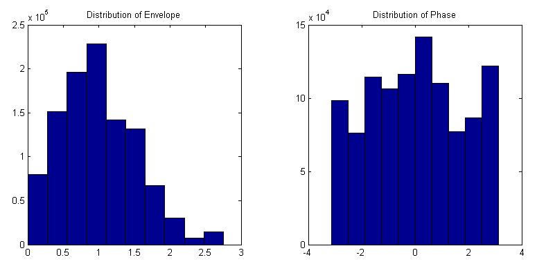
The above code was used to generate Rayleigh sequences of varying lengths with Doppler frequencies of 5 Hz, 70 Hz and 300 Hz. The sampling frequency was fixed at 7.68 MHz (corresponding to a BW of 5 MHz). It must be noted that in this simulation the length of the Gaussian sequence is equal to the filter length in the frequency domain. It was found that to generate a Rayleigh sequence of reasonable length the length of the Gaussian sequence has to be quite large (2^20 in the above example). As before we calculated the distribution of envelope and phase of the generated sequence as well as the LCR and AFD. These were found to be within reasonable margins.

Note:

1. Level crossing rate (LCR) is defined as number of times per second the signal envelope crosses a given threshold. This could be either in the positive direction or negative direction.
2. Average fade duration (AFD) is the average duration that the signal envelope remains below a given threshold once it crosses that threshold. Simply it is the average duration of a fading event.
3. The LCR and AFD are interconnected and the product of these two quantities is a constant.

[1] David J. Young and Norman C. Beaulieu, "The Generation of Correlated Rayleigh Random Variates by Inverse Discrete Fourier Transform", IEEE Transactions on Communications vol. 48 no. 7 July 2000.

Author: Yasir Ahmed (aka John)

More than 20 years of experience in various organizations in Pakistan, the USA, and Europe. Worked as a Research Assistant within the Mobile and Portable Radio Group (MPRG) of Virginia Tech and was one of the first researchers to propose Space Time Block Codes for eight transmit antennas. The collaboration with MPRG continued even after graduating with an MSEE degree and has resulted in 12 research publications and a book on Wireless Communications. Worked for Qualcomm USA as an Engineer with the key role of performance and conformance testing of UMTS modems. Qualcomm is the inventor of CDMA technology and owns patents critical to the 4G and 5G standards.

Twitter Facebook Linkedin